Methods and tools for efficient training on a single GPU

This guide demonstrates practical techniques that you can use to increase the efficiency of your model’s training by optimizing memory utilization, speeding up the training, or both. If you’d like to understand how GPU is utilized during training, please refer to the Model training anatomy conceptual guide first. This guide focuses on practical techniques.

If you have access to a machine with multiple GPUs, these approaches are still valid, plus you can leverage additional methods outlined in the multi-GPU section.

When training large models, there are two aspects that should be considered at the same time:

• Data throughput/training time

• Model performance

Maximizing the throughput (samples/second) leads to lower training cost. This is generally achieved by utilizing the GPU as much as possible and thus filling GPU memory to its limit. If the desired batch size exceeds the limits of the GPU memory, the memory optimization techniques, such as gradient accumulation, can help.

However, if the preferred batch size fits into memory, there’s no reason to apply memory-optimizing techniques because they can slow down the training. Just because one can use a large batch size, does not necessarily mean they should. As part of hyperparameter tuning, you should determine which batch size yields the best results and then optimize resources accordingly.

The methods and tools covered in this guide can be classified based on the effect they have on the training process:

Method/tool	Improves training speed	Optimizes memory utilization
Batch size choice	Yes	Yes
Gradient accumulation	No	Yes
Gradient checkpointing	No	Yes
Mixed precision training	Yes	(No)
Optimizer choice	Yes	Yes
Data preloading	Yes	No
DeepSpeed Zero	No	Yes
torch.compile	Yes	No

Note: when using mixed precision with a small model and a large batch size, there will be some memory savings but with a large model and a small batch size, the memory use will be larger.

You can combine the above methods to get a cumulative effect. These techniques are available to you whether you are training your model with Trainer or writing a pure PyTorch loop, in which case you can configure these optimizations with 🌍 Accelerate.

If these methods do not result in sufficient gains, you can explore the following options:

• Look into building your own custom Docker container with efficient softare prebuilds

• Consider a model that uses Mixture of Experts (MoE)

• Convert your model to BetterTransformer to leverage PyTorch native attention

Finally, if all of the above is still not enough, even after switching to a server-grade GPU like A100, consider moving to a multi-GPU setup. All these approaches are still valid in a multi-GPU setup, plus you can leverage additional parallelism techniques outlined in the multi-GPU section.

Batch size choice

To achieve optimal performance, start by identifying the appropriate batch size. It is recommended to use batch sizes and input/output neuron counts that are of size 2^N. Often it’s a multiple of 8, but it can be higher depending on the hardware being used and the model’s dtype.

For reference, check out NVIDIA’s recommendation for input/output neuron counts and batch size for fully connected layers (which are involved in GEMMs (General Matrix Multiplications)).

Tensor Core Requirements define the multiplier based on the dtype and the hardware. For instance, for fp16 data type a multiple of 8 is recommended, unless it’s an A100 GPU, in which case use multiples of 64.

For parameters that are small, consider also Dimension Quantization Effects. This is where tiling happens and the right multiplier can have a significant speedup.

Gradient Accumulation

The gradient accumulation method aims to calculate gradients in smaller increments instead of computing them for the entire batch at once. This approach involves iteratively calculating gradients in smaller batches by performing forward and backward passes through the model and accumulating the gradients during the process. Once a sufficient number of gradients have been accumulated, the model’s optimization step is executed. By employing gradient accumulation, it becomes possible to increase the effective batch size beyond the limitations imposed by the GPU’s memory capacity. However, it is important to note that the additional forward and backward passes introduced by gradient accumulation can slow down the training process.

You can enable gradient accumulation by adding the gradient_accumulation_steps argument to TrainingArguments:

Copied

training_args = TrainingArguments(per_device_train_batch_size=1, gradient_accumulation_steps=4, **default_args)

In the above example, your effective batch size becomes 4.

Alternatively, use 🌍 Accelerate to gain full control over the training loop. Find the 🌍 Accelerate example further down in this guide.

While it is advised to max out GPU usage as much as possible, a high number of gradient accumulation steps can result in a more pronounced training slowdown. Consider the following example. Let’s say, the per_device_train_batch_size=4 without gradient accumulation hits the GPU’s limit. If you would like to train with batches of size 64, do not set the per_device_train_batch_size to 1 and gradient_accumulation_steps to 64. Instead, keep per_device_train_batch_size=4 and set gradient_accumulation_steps=16. This results in the same effective batch size while making better use of the available GPU resources.

For additional information, please refer to batch size and gradient accumulation benchmarks for RTX-3090 and A100.

Gradient Checkpointing

Some large models may still face memory issues even when the batch size is set to 1 and gradient accumulation is used. This is because there are other components that also require memory storage.

Saving all activations from the forward pass in order to compute the gradients during the backward pass can result in significant memory overhead. The alternative approach of discarding the activations and recalculating them when needed during the backward pass, would introduce a considerable computational overhead and slow down the training process.

Gradient checkpointing offers a compromise between these two approaches and saves strategically selected activations throughout the computational graph so only a fraction of the activations need to be re-computed for the gradients. For an in-depth explanation of gradient checkpointing, refer to this great article.

To enable gradient checkpointing in the Trainer, pass the corresponding a flag to TrainingArguments:

Copied

training_args = TrainingArguments(
    per_device_train_batch_size=1, gradient_accumulation_steps=4, gradient_checkpointing=True, **default_args
)

Alternatively, use 🌍 Accelerate - find the 🌍 Accelerate example further in this guide.

While gradient checkpointing may improve memory efficiency, it slows training by approximately 20%.

Mixed precision training

Mixed precision training is a technique that aims to optimize the computational efficiency of training models by utilizing lower-precision numerical formats for certain variables. Traditionally, most models use 32-bit floating point precision (fp32 or float32) to represent and process variables. However, not all variables require this high precision level to achieve accurate results. By reducing the precision of certain variables to lower numerical formats like 16-bit floating point (fp16 or float16), we can speed up the computations. Because in this approach some computations are performed in half-precision, while some are still in full precision, the approach is called mixed precision training.

Most commonly mixed precision training is achieved by using fp16 (float16) data types, however, some GPU architectures (such as the Ampere architecture) offer bf16 and tf32 (CUDA internal data type) data types. Check out the NVIDIA Blog to learn more about the differences between these data types.

fp16

The main advantage of mixed precision training comes from saving the activations in half precision (fp16). Although the gradients are also computed in half precision they are converted back to full precision for the optimization step so no memory is saved here. While mixed precision training results in faster computations, it can also lead to more GPU memory being utilized, especially for small batch sizes. This is because the model is now present on the GPU in both 16-bit and 32-bit precision (1.5x the original model on the GPU).

To enable mixed precision training, set the fp16 flag to True:

Copied

training_args = TrainingArguments(per_device_train_batch_size=4, fp16=True, **default_args)

If you prefer to use 🌍 Accelerate, find the 🌍 Accelerate example further in this guide.

BF16

If you have access to an Ampere or newer hardware you can use bf16 for mixed precision training and evaluation. While bf16 has a worse precision than fp16, it has a much bigger dynamic range. In fp16 the biggest number you can have is 65535 and any number above that will result in an overflow. A bf16 number can be as large as 3.39e+38 (!) which is about the same as fp32 - because both have 8-bits used for the numerical range.

You can enable BF16 in the 🌍 Trainer with:

Copied

training_args = TrainingArguments(bf16=True, **default_args)

TF32

The Ampere hardware uses a magical data type called tf32. It has the same numerical range as fp32 (8-bits), but instead of 23 bits precision it has only 10 bits (same as fp16) and uses only 19 bits in total. It’s “magical” in the sense that you can use the normal fp32 training and/or inference code and by enabling tf32 support you can get up to 3x throughput improvement. All you need to do is to add the following to your code:

Copied

import torch
torch.backends.cuda.matmul.allow_tf32 = True
torch.backends.cudnn.allow_tf32 = True

CUDA will automatically switch to using tf32 instead of fp32 where possible, assuming that the used GPU is from the Ampere series.

According to NVIDIA research, the majority of machine learning training workloads show the same perplexity and convergence with tf32 training as with fp32. If you’re already using fp16 or bf16 mixed precision it may help with the throughput as well.

You can enable this mode in the 🌍 Trainer:

Copied

TrainingArguments(tf32=True, **default_args)

tf32 can’t be accessed directly via tensor.to(dtype=torch.tf32) because it is an internal CUDA data type. You need torch>=1.7 to use tf32 data types.

For additional information on tf32 vs other precisions, please refer to the following benchmarks: RTX-3090 and A100.

Flash Attention 2

You can speedup the training throughput by using Flash Attention 2 integration in transformers. Check out the appropriate section in the single GPU section to learn more about how to load a model with Flash Attention 2 modules.

Optimizer choice

The most common optimizer used to train transformer models is Adam or AdamW (Adam with weight decay). Adam achieves good convergence by storing the rolling average of the previous gradients; however, it adds an additional memory footprint of the order of the number of model parameters. To remedy this, you can use an alternative optimizer. For example if you have NVIDIA/apex installed, adamw_apex_fused will give you the fastest training experience among all supported AdamW optimizers.

Trainer integrates a variety of optimizers that can be used out of box: adamw_hf, adamw_torch, adamw_torch_fused, adamw_apex_fused, adamw_anyprecision, adafactor, or adamw_bnb_8bit. More optimizers can be plugged in via a third-party implementation.

Let’s take a closer look at two alternatives to AdamW optimizer:

1. adafactor which is available in Trainer

2. adamw_bnb_8bit is also available in Trainer, but a third-party integration is provided below for demonstration.

For comparison, for a 3B-parameter model, like “t5-3b”:

• A standard AdamW optimizer will need 24GB of GPU memory because it uses 8 bytes for each parameter (8*3 => 24GB)

• Adafactor optimizer will need more than 12GB. It uses slightly more than 4 bytes for each parameter, so 4*3 and then some extra.

• 8bit BNB quantized optimizer will use only (2*3) 6GB if all optimizer states are quantized.

Adafactor

Adafactor doesn’t store rolling averages for each element in weight matrices. Instead, it keeps aggregated information (sums of rolling averages row- and column-wise), significantly reducing its footprint. However, compared to Adam, Adafactor may have slower convergence in certain cases.

You can switch to Adafactor by setting optim="adafactor" in TrainingArguments:

Copied

training_args = TrainingArguments(per_device_train_batch_size=4, optim="adafactor", **default_args)

Combined with other approaches (gradient accumulation, gradient checkpointing, and mixed precision training) you can notice up to 3x improvement while maintaining the throughput! However, as mentioned before, the convergence of Adafactor can be worse than Adam.

8-bit Adam

Instead of aggregating optimizer states like Adafactor, 8-bit Adam keeps the full state and quantizes it. Quantization means that it stores the state with lower precision and dequantizes it only for the optimization. This is similar to the idea behind mixed precision training.

To use adamw_bnb_8bit, you simply need to set optim="adamw_bnb_8bit" in TrainingArguments:

Copied

training_args = TrainingArguments(per_device_train_batch_size=4, optim="adamw_bnb_8bit", **default_args)

However, we can also use a third-party implementation of the 8-bit optimizer for demonstration purposes to see how that can be integrated.

First, follow the installation guide in the GitHub repo to install the bitsandbytes library that implements the 8-bit Adam optimizer.

Next you need to initialize the optimizer. This involves two steps:

• First, group the model’s parameters into two groups - one where weight decay should be applied, and the other one where it should not. Usually, biases and layer norm parameters are not weight decayed.

• Then do some argument housekeeping to use the same parameters as the previously used AdamW optimizer.

Copied

import bitsandbytes as bnb
from torch import nn
from transformers.trainer_pt_utils import get_parameter_names

training_args = TrainingArguments(per_device_train_batch_size=4, **default_args)

decay_parameters = get_parameter_names(model, [nn.LayerNorm])
decay_parameters = [name for name in decay_parameters if "bias" not in name]
optimizer_grouped_parameters = [
    {
        "params": [p for n, p in model.named_parameters() if n in decay_parameters],
        "weight_decay": training_args.weight_decay,
    },
    {
        "params": [p for n, p in model.named_parameters() if n not in decay_parameters],
        "weight_decay": 0.0,
    },
]

optimizer_kwargs = {
    "betas": (training_args.adam_beta1, training_args.adam_beta2),
    "eps": training_args.adam_epsilon,
}
optimizer_kwargs["lr"] = training_args.learning_rate
adam_bnb_optim = bnb.optim.Adam8bit(
    optimizer_grouped_parameters,
    betas=(training_args.adam_beta1, training_args.adam_beta2),
    eps=training_args.adam_epsilon,
    lr=training_args.learning_rate,
)

Finally, pass the custom optimizer as an argument to the Trainer:

Copied

trainer = Trainer(model=model, args=training_args, train_dataset=ds, optimizers=(adam_bnb_optim, None))

Combined with other approaches (gradient accumulation, gradient checkpointing, and mixed precision training), you can expect to get about a 3x memory improvement and even slightly higher throughput as using Adafactor.

multi_tensor

pytorch-nightly introduced torch.optim._multi_tensor which should significantly speed up the optimizers for situations with lots of small feature tensors. It should eventually become the default, but if you want to experiment with it sooner, take a look at this GitHub issue.

Data preloading

One of the important requirements to reach great training speed is the ability to feed the GPU at the maximum speed it can handle. By default, everything happens in the main process, and it might not be able to read the data from disk fast enough, and thus create a bottleneck, leading to GPU under-utilization. Configure the following arguments to reduce the bottleneck:

• DataLoader(pin_memory=True, ...) - ensures the data gets preloaded into the pinned memory on CPU and typically leads to much faster transfers from CPU to GPU memory.

• DataLoader(num_workers=4, ...) - spawn several workers to preload data faster. During training, watch the GPU utilization stats; if it’s far from 100%, experiment with increasing the number of workers. Of course, the problem could be elsewhere, so many workers won’t necessarily lead to better performance.

When using Trainer, the corresponding TrainingArguments are: dataloader_pin_memory (True by default), and dataloader_num_workers (defaults to 0).

DeepSpeed ZeRO

DeepSpeed is an open-source deep learning optimization library that is integrated with 🌍 Transformers and 🌍 Accelerate. It provides a wide range of features and optimizations designed to improve the efficiency and scalability of large-scale deep learning training.

If your model fits onto a single GPU and you have enough space to fit a small batch size, you don’t need to use DeepSpeed as it’ll only slow things down. However, if the model doesn’t fit onto a single GPU or you can’t fit a small batch, you can leverage DeepSpeed ZeRO + CPU Offload, or NVMe Offload for much larger models. In this case, you need to separately install the library, then follow one of the guides to create a configuration file and launch DeepSpeed:

• For an in-depth guide on DeepSpeed integration with Trainer, review the corresponding documentation, specifically the section for a single GPU. Some adjustments are required to use DeepSpeed in a notebook; please take a look at the corresponding guide.

• If you prefer to use 🌍 Accelerate, refer to 🌍 Accelerate DeepSpeed guide.

Using torch.compile

PyTorch 2.0 introduced a new compile function that doesn’t require any modification to existing PyTorch code but can optimize your code by adding a single line of code: model = torch.compile(model).

If using Trainer, you only need to pass the torch_compile option in the TrainingArguments:

Copied

training_args = TrainingArguments(torch_compile=True, **default_args)

torch.compile uses Python’s frame evaluation API to automatically create a graph from existing PyTorch programs. After capturing the graph, different backends can be deployed to lower the graph to an optimized engine. You can find more details and benchmarks in PyTorch documentation.

torch.compile has a growing list of backends, which can be found in by calling torchdynamo.list_backends(), each of which with its optional dependencies.

Choose which backend to use by specifying it via torch_compile_backend in the TrainingArguments. Some of the most commonly used backends are:

Debugging backends:

• dynamo.optimize("eager") - Uses PyTorch to run the extracted GraphModule. This is quite useful in debugging TorchDynamo issues.

• dynamo.optimize("aot_eager") - Uses AotAutograd with no compiler, i.e, just using PyTorch eager for the AotAutograd’s extracted forward and backward graphs. This is useful for debugging, and unlikely to give speedups.

Training & inference backends:

• dynamo.optimize("inductor") - Uses TorchInductor backend with AotAutograd and cudagraphs by leveraging codegened Triton kernels Read more

• dynamo.optimize("nvfuser") - nvFuser with TorchScript. Read more

• dynamo.optimize("aot_nvfuser") - nvFuser with AotAutograd. Read more

• dynamo.optimize("aot_cudagraphs") - cudagraphs with AotAutograd. Read more

Inference-only backends:

• dynamo.optimize("ofi") - Uses Torchscript optimize_for_inference. Read more

• dynamo.optimize("fx2trt") - Uses Nvidia TensorRT for inference optimizations. Read more

• dynamo.optimize("onnxrt") - Uses ONNXRT for inference on CPU/GPU. Read more

• dynamo.optimize("ipex") - Uses IPEX for inference on CPU. Read more

For an example of using torch.compile with 🌍 Transformers, check out this blog post on fine-tuning a BERT model for Text Classification using the newest PyTorch 2.0 features

Using 🌍 Accelerate

With 🌍 Accelerate you can use the above methods while gaining full control over the training loop and can essentially write the loop in pure PyTorch with some minor modifications.

Suppose you have combined the methods in the TrainingArguments like so:

Copied

training_args = TrainingArguments(
    per_device_train_batch_size=1,
    gradient_accumulation_steps=4,
    gradient_checkpointing=True,
    fp16=True,
    **default_args,
)

The full example training loop with 🌍 Accelerate is only a handful of lines of code long:

Copied

from accelerate import Accelerator
from torch.utils.data.dataloader import DataLoader

dataloader = DataLoader(ds, batch_size=training_args.per_device_train_batch_size)

if training_args.gradient_checkpointing:
    model.gradient_checkpointing_enable()

accelerator = Accelerator(fp16=training_args.fp16)
model, optimizer, dataloader = accelerator.prepare(model, adam_bnb_optim, dataloader)

model.train()
for step, batch in enumerate(dataloader, start=1):
    loss = model(**batch).loss
    loss = loss / training_args.gradient_accumulation_steps
    accelerator.backward(loss)
    if step % training_args.gradient_accumulation_steps == 0:
        optimizer.step()
        optimizer.zero_grad()

First we wrap the dataset in a DataLoader. Then we can enable gradient checkpointing by calling the model’s gradient_checkpointing_enable() method. When we initialize the Accelerator we can specify if we want to use mixed precision training and it will take care of it for us in the prepare call. During the prepare call the dataloader will also be distributed across workers should we use multiple GPUs. We use the same 8-bit optimizer from the earlier example.

Finally, we can add the main training loop. Note that the backward call is handled by 🌍 Accelerate. We can also see how gradient accumulation works: we normalize the loss, so we get the average at the end of accumulation and once we have enough steps we run the optimization.

Implementing these optimization techniques with 🌍 Accelerate only takes a handful of lines of code and comes with the benefit of more flexibility in the training loop. For a full documentation of all features have a look at the Accelerate documentation.

Efficient Software Prebuilds

PyTorch’s pip and conda builds come prebuilt with the cuda toolkit which is enough to run PyTorch, but it is insufficient if you need to build cuda extensions.

At times, additional efforts may be required to pre-build some components. For instance, if you’re using libraries like apex that don’t come pre-compiled. In other situations figuring out how to install the right cuda toolkit system-wide can be complicated. To address these scenarios PyTorch and NVIDIA released a new version of NGC docker container which already comes with everything prebuilt. You just need to install your programs on it, and it will run out of the box.

This approach is also useful if you want to tweak the pytorch source and/or make a new customized build. To find the docker image version you want start with PyTorch release notes, choose one of the latest monthly releases. Go into the release’s notes for the desired release, check that the environment’s components are matching your needs (including NVIDIA Driver requirements!) and then at the very top of that document go to the corresponding NGC page. If for some reason you get lost, here is the index of all PyTorch NGC images.

Next follow the instructions to download and deploy the docker image.

Mixture of Experts

Some recent papers reported a 4-5x training speedup and a faster inference by integrating Mixture of Experts (MoE) into the Transformer models.

Since it has been discovered that more parameters lead to better performance, this technique allows to increase the number of parameters by an order of magnitude without increasing training costs.

In this approach every other FFN layer is replaced with a MoE Layer which consists of many experts, with a gated function that trains each expert in a balanced way depending on the input token’s position in a sequence.

MoE Transformer 2x block

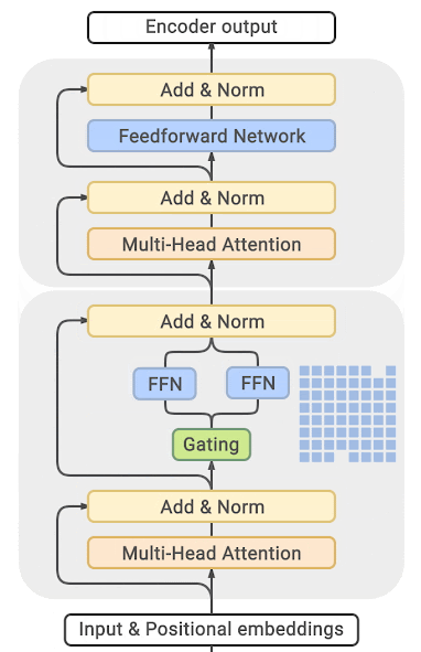
(source: GLAM)

You can find exhaustive details and comparison tables in the papers listed at the end of this section.

The main drawback of this approach is that it requires staggering amounts of GPU memory - almost an order of magnitude larger than its dense equivalent. Various distillation and approaches are proposed to how to overcome the much higher memory requirements.

There is direct trade-off though, you can use just a few experts with a 2-3x smaller base model instead of dozens or hundreds experts leading to a 5x smaller model and thus increase the training speed moderately while increasing the memory requirements moderately as well.

Most related papers and implementations are built around Tensorflow/TPUs:

• GShard: Scaling Giant Models with Conditional Computation and Automatic Sharding

• Switch Transformers: Scaling to Trillion Parameter Models with Simple and Efficient Sparsity

• GLaM: Generalist Language Model (GLaM)

And for Pytorch DeepSpeed has built one as well: DeepSpeed-MoE: Advancing Mixture-of-Experts Inference and Training to Power Next-Generation AI Scale, Mixture of Experts - blog posts: 1, 2 and specific deployment with large transformer-based natural language generation models: blog post, Megatron-Deepspeed branch.

Using PyTorch native attention and Flash Attention

PyTorch 2.0 released a native torch.nn.functional.scaled_dot_product_attention (SDPA), that allows using fused GPU kernels such as memory-efficient attention and flash attention.

After installing the optimum package, the relevant internal modules can be replaced to use PyTorch’s native attention with:

Copied

model = model.to_bettertransformer()

Once converted, train the model as usual.

The PyTorch-native scaled_dot_product_attention operator can only dispatch to Flash Attention if no attention_mask is provided.

By default, in training mode, the BetterTransformer integration drops the mask support and can only be used for training that does not require a padding mask for batched training. This is the case, for example, during masked language modeling or causal language modeling. BetterTransformer is not suited for fine-tuning models on tasks that require a padding mask.

Check out this blogpost to learn more about acceleration and memory-savings with SDPA.