Evaluating Diffusion Models

Evaluating Diffusion Models

Evaluation of generative models like Stable Diffusion is subjective in nature. But as practitioners and researchers, we often have to make careful choices amongst many different possibilities. So, when working with different generative models (like GANs, Diffusion, etc.), how do we choose one over the other?

Qualitative evaluation of such models can be error-prone and might incorrectly influence a decision. However, quantitative metrics don’t necessarily correspond to image quality. So, usually, a combination of both qualitative and quantitative evaluations provides a stronger signal when choosing one model over the other.

In this document, we provide a non-exhaustive overview of qualitative and quantitative methods to evaluate Diffusion models. For quantitative methods, we specifically focus on how to implement them alongside diffusers.

The methods shown in this document can also be used to evaluate different noise schedulers keeping the underlying generation model fixed.

Scenarios

We cover Diffusion models with the following pipelines:

• Text-guided image generation (such as the StableDiffusionPipeline).

• Text-guided image generation, additionally conditioned on an input image (such as the StableDiffusionImg2ImgPipeline, and StableDiffusionInstructPix2PixPipeline).

• Class-conditioned image generation models (such as the DiTPipeline).

Qualitative Evaluation

Qualitative evaluation typically involves human assessment of generated images. Quality is measured across aspects such as compositionality, image-text alignment, and spatial relations. Common prompts provide a degree of uniformity for subjective metrics. DrawBench and PartiPrompts are prompt datasets used for qualitative benchmarking. DrawBench and PartiPrompts were introduced by Imagen and Parti respectively.

From the official Parti website:

PartiPrompts (P2) is a rich set of over 1600 prompts in English that we release as part of this work. P2 can be used to measure model capabilities across various categories and challenge aspects.

parti-prompts

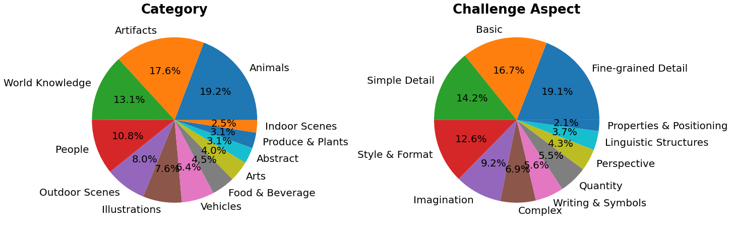
PartiPrompts has the following columns:

• Prompt

• Category of the prompt (such as “Abstract”, “World Knowledge”, etc.)

• Challenge reflecting the difficulty (such as “Basic”, “Complex”, “Writing & Symbols”, etc.)

These benchmarks allow for side-by-side human evaluation of different image generation models.

For this, the 🧨 Diffusers team has built Open Parti Prompts, which is a community-driven qualitative benchmark based on Parti Prompts to compare state-of-the-art open-source diffusion models:

• Open Parti Prompts Game: For 10 parti prompts, 4 generated images are shown and the user selects the image that suits the prompt best.
• Open Parti Prompts Leaderboard: The leaderboard comparing the currently best open-sourced diffusion models to each other.

To manually compare images, let’s see how we can use diffusers on a couple of PartiPrompts.

Below we show some prompts sampled across different challenges: Basic, Complex, Linguistic Structures, Imagination, and Writing & Symbols. Here we are using PartiPrompts as a dataset.

Copied

from datasets import load_dataset

# prompts = load_dataset("nateraw/parti-prompts", split="train")
# prompts = prompts.shuffle()
# sample_prompts = [prompts[i]["Prompt"] for i in range(5)]

# Fixing these sample prompts in the interest of reproducibility.
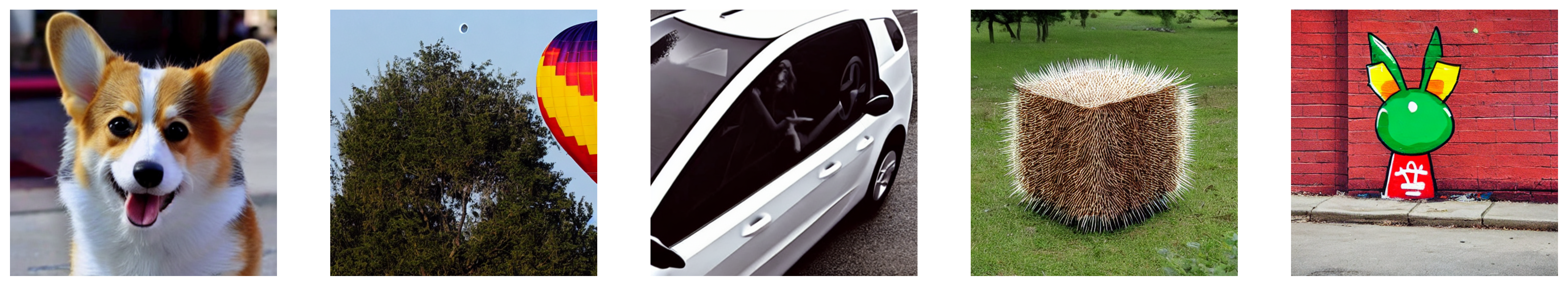
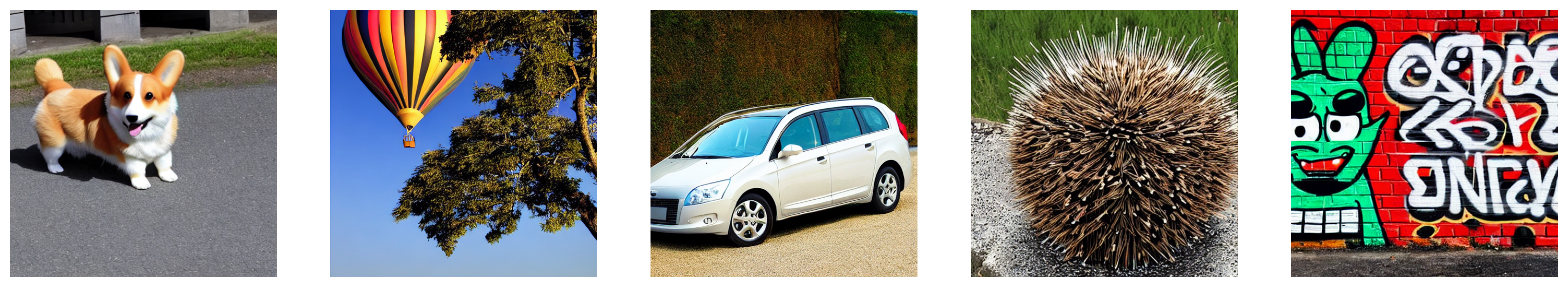
sample_prompts = [
    "a corgi",
    "a hot air balloon with a yin-yang symbol, with the moon visible in the daytime sky",
    "a car with no windows",
    "a cube made of porcupine",
    'The saying "BE EXCELLENT TO EACH OTHER" written on a red brick wall with a graffiti image of a green alien wearing a tuxedo. A yellow fire hydrant is on a sidewalk in the foreground.',
]

Now we can use these prompts to generate some images using Stable Diffusion (v1-4 checkpoint):

Copied

import torch

seed = 0
generator = torch.manual_seed(seed)

images = sd_pipeline(sample_prompts, num_images_per_prompt=1, generator=generator, output_type="numpy").images

parti-prompts-14

We can also set num_images_per_prompt accordingly to compare different images for the same prompt. Running the same pipeline but with a different checkpoint (v1-5), yields:

parti-prompts-15

Once several images are generated from all the prompts using multiple models (under evaluation), these results are presented to human evaluators for scoring. For more details on the DrawBench and PartiPrompts benchmarks, refer to their respective papers.

It is useful to look at some inference samples while a model is training to measure the training progress. In our training scripts, we support this utility with additional support for logging to TensorBoard and Weights & Biases.

Quantitative Evaluation

In this section, we will walk you through how to evaluate three different diffusion pipelines using:

• CLIP score

• CLIP directional similarity

• FID

Text-guided image generation

CLIP score measures the compatibility of image-caption pairs. Higher CLIP scores imply higher compatibility 🔼. The CLIP score is a quantitative measurement of the qualitative concept “compatibility”. Image-caption pair compatibility can also be thought of as the semantic similarity between the image and the caption. CLIP score was found to have high correlation with human judgement.

Let’s first load a StableDiffusionPipeline:

Copied

from diffusers import StableDiffusionPipeline
import torch

model_ckpt = "CompVis/stable-diffusion-v1-4"
sd_pipeline = StableDiffusionPipeline.from_pretrained(model_ckpt, torch_dtype=torch.float16).to("cuda")

Generate some images with multiple prompts:

Copied

prompts = [
    "a photo of an astronaut riding a horse on mars",
    "A high tech solarpunk utopia in the Amazon rainforest",
    "A pikachu fine dining with a view to the Eiffel Tower",
    "A mecha robot in a favela in expressionist style",
    "an insect robot preparing a delicious meal",
    "A small cabin on top of a snowy mountain in the style of Disney, artstation",
]

images = sd_pipeline(prompts, num_images_per_prompt=1, output_type="numpy").images

print(images.shape)
# (6, 512, 512, 3)

And then, we calculate the CLIP score.

Copied

from torchmetrics.functional.multimodal import clip_score
from functools import partial

clip_score_fn = partial(clip_score, model_name_or_path="openai/clip-vit-base-patch16")


def calculate_clip_score(images, prompts):
    images_int = (images * 255).astype("uint8")
    clip_score = clip_score_fn(torch.from_numpy(images_int).permute(0, 3, 1, 2), prompts).detach()
    return round(float(clip_score), 4)


sd_clip_score = calculate_clip_score(images, prompts)
print(f"CLIP score: {sd_clip_score}")
# CLIP score: 35.7038

In the above example, we generated one image per prompt. If we generated multiple images per prompt, we would have to take the average score from the generated images per prompt.

Now, if we wanted to compare two checkpoints compatible with the StableDiffusionPipeline we should pass a generator while calling the pipeline. First, we generate images with a fixed seed with the v1-4 Stable Diffusion checkpoint:

Copied

seed = 0
generator = torch.manual_seed(seed)

images = sd_pipeline(prompts, num_images_per_prompt=1, generator=generator, output_type="numpy").images

Then we load the v1-5 checkpoint to generate images:

Copied

model_ckpt_1_5 = "runwayml/stable-diffusion-v1-5"
sd_pipeline_1_5 = StableDiffusionPipeline.from_pretrained(model_ckpt_1_5, torch_dtype=weight_dtype).to(device)

images_1_5 = sd_pipeline_1_5(prompts, num_images_per_prompt=1, generator=generator, output_type="numpy").images

And finally, we compare their CLIP scores:

Copied

sd_clip_score_1_4 = calculate_clip_score(images, prompts)
print(f"CLIP Score with v-1-4: {sd_clip_score_1_4}")
# CLIP Score with v-1-4: 34.9102

sd_clip_score_1_5 = calculate_clip_score(images_1_5, prompts)
print(f"CLIP Score with v-1-5: {sd_clip_score_1_5}")
# CLIP Score with v-1-5: 36.2137

It seems like the v1-5 checkpoint performs better than its predecessor. Note, however, that the number of prompts we used to compute the CLIP scores is quite low. For a more practical evaluation, this number should be way higher, and the prompts should be diverse.

By construction, there are some limitations in this score. The captions in the training dataset were crawled from the web and extracted from alt and similar tags associated an image on the internet. They are not necessarily representative of what a human being would use to describe an image. Hence we had to “engineer” some prompts here.

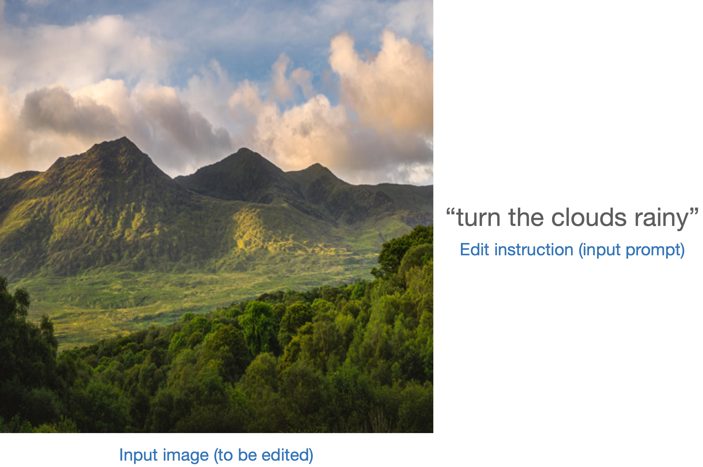
Image-conditioned text-to-image generation

In this case, we condition the generation pipeline with an input image as well as a text prompt. Let’s take the StableDiffusionInstructPix2PixPipeline, as an example. It takes an edit instruction as an input prompt and an input image to be edited.

Here is one example:

edit-instruction

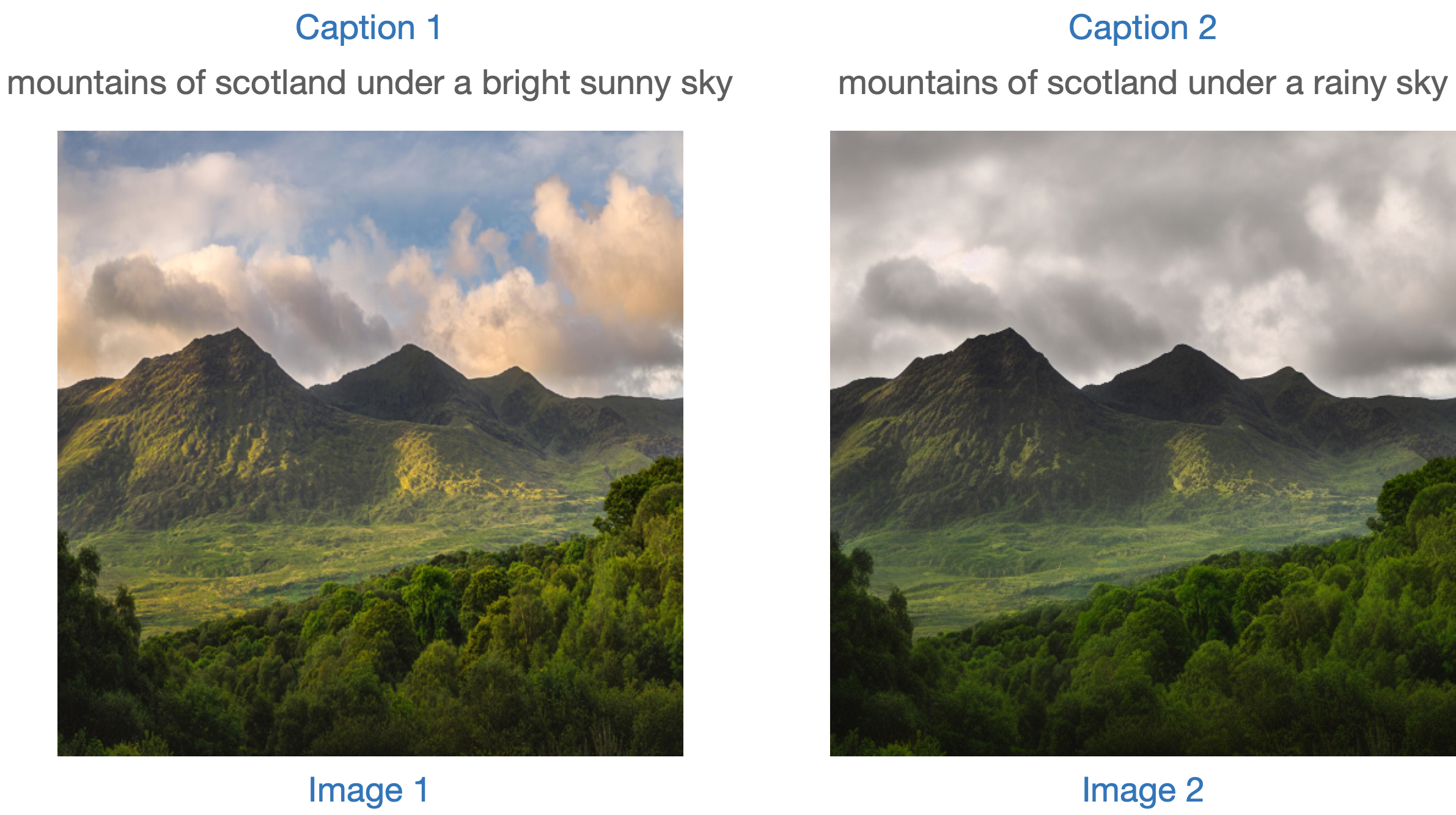
One strategy to evaluate such a model is to measure the consistency of the change between the two images (in CLIP space) with the change between the two image captions (as shown in CLIP-Guided Domain Adaptation of Image Generators). This is referred to as the ”CLIP directional similarity“.

• Caption 1 corresponds to the input image (image 1) that is to be edited.

• Caption 2 corresponds to the edited image (image 2). It should reflect the edit instruction.

Following is a pictorial overview:

edit-consistency

We have prepared a mini dataset to implement this metric. Let’s first load the dataset.

Copied

from datasets import load_dataset

dataset = load_dataset("sayakpaul/instructpix2pix-demo", split="train")
dataset.features

Copied

{'input': Value(dtype='string', id=None),
 'edit': Value(dtype='string', id=None),
 'output': Value(dtype='string', id=None),
 'image': Image(decode=True, id=None)}

Here we have:

• input is a caption corresponding to the image.

• edit denotes the edit instruction.

• output denotes the modified caption reflecting the edit instruction.

Let’s take a look at a sample.

Copied

idx = 0
print(f"Original caption: {dataset[idx]['input']}")
print(f"Edit instruction: {dataset[idx]['edit']}")
print(f"Modified caption: {dataset[idx]['output']}")

Copied

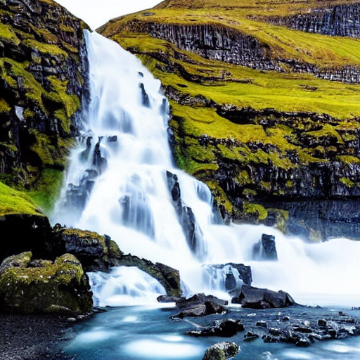
Original caption: 2. FAROE ISLANDS: An archipelago of 18 mountainous isles in the North Atlantic Ocean between Norway and Iceland, the Faroe Islands has 'everything you could hope for', according to Big 7 Travel. It boasts 'crystal clear waterfalls, rocky cliffs that seem to jut out of nowhere and velvety green hills'
Edit instruction: make the isles all white marble
Modified caption: 2. WHITE MARBLE ISLANDS: An archipelago of 18 mountainous white marble isles in the North Atlantic Ocean between Norway and Iceland, the White Marble Islands has 'everything you could hope for', according to Big 7 Travel. It boasts 'crystal clear waterfalls, rocky cliffs that seem to jut out of nowhere and velvety green hills'

And here is the image:

Copied

dataset[idx]["image"]

edit-dataset

We will first edit the images of our dataset with the edit instruction and compute the directional similarity.

Let’s first load the StableDiffusionInstructPix2PixPipeline:

Copied

from diffusers import StableDiffusionInstructPix2PixPipeline

instruct_pix2pix_pipeline = StableDiffusionInstructPix2PixPipeline.from_pretrained(
    "timbrooks/instruct-pix2pix", torch_dtype=torch.float16
).to(device)

Now, we perform the edits:

Copied

import numpy as np


def edit_image(input_image, instruction):
    image = instruct_pix2pix_pipeline(
        instruction,
        image=input_image,
        output_type="numpy",
        generator=generator,
    ).images[0]
    return image


input_images = []
original_captions = []
modified_captions = []
edited_images = []

for idx in range(len(dataset)):
    input_image = dataset[idx]["image"]
    edit_instruction = dataset[idx]["edit"]
    edited_image = edit_image(input_image, edit_instruction)

    input_images.append(np.array(input_image))
    original_captions.append(dataset[idx]["input"])
    modified_captions.append(dataset[idx]["output"])
    edited_images.append(edited_image)

To measure the directional similarity, we first load CLIP’s image and text encoders:

Copied

from transformers import (
    CLIPTokenizer,
    CLIPTextModelWithProjection,
    CLIPVisionModelWithProjection,
    CLIPImageProcessor,
)

clip_id = "openai/clip-vit-large-patch14"
tokenizer = CLIPTokenizer.from_pretrained(clip_id)
text_encoder = CLIPTextModelWithProjection.from_pretrained(clip_id).to(device)
image_processor = CLIPImageProcessor.from_pretrained(clip_id)
image_encoder = CLIPVisionModelWithProjection.from_pretrained(clip_id).to(device)

Notice that we are using a particular CLIP checkpoint, i.e., openai/clip-vit-large-patch14. This is because the Stable Diffusion pre-training was performed with this CLIP variant. For more details, refer to the documentation.

Next, we prepare a PyTorch nn.Module to compute directional similarity:

Copied

import torch.nn as nn
import torch.nn.functional as F


class DirectionalSimilarity(nn.Module):
    def __init__(self, tokenizer, text_encoder, image_processor, image_encoder):
        super().__init__()
        self.tokenizer = tokenizer
        self.text_encoder = text_encoder
        self.image_processor = image_processor
        self.image_encoder = image_encoder

    def preprocess_image(self, image):
        image = self.image_processor(image, return_tensors="pt")["pixel_values"]
        return {"pixel_values": image.to(device)}

    def tokenize_text(self, text):
        inputs = self.tokenizer(
            text,
            max_length=self.tokenizer.model_max_length,
            padding="max_length",
            truncation=True,
            return_tensors="pt",
        )
        return {"input_ids": inputs.input_ids.to(device)}

    def encode_image(self, image):
        preprocessed_image = self.preprocess_image(image)
        image_features = self.image_encoder(**preprocessed_image).image_embeds
        image_features = image_features / image_features.norm(dim=1, keepdim=True)
        return image_features

    def encode_text(self, text):
        tokenized_text = self.tokenize_text(text)
        text_features = self.text_encoder(**tokenized_text).text_embeds
        text_features = text_features / text_features.norm(dim=1, keepdim=True)
        return text_features

    def compute_directional_similarity(self, img_feat_one, img_feat_two, text_feat_one, text_feat_two):
        sim_direction = F.cosine_similarity(img_feat_two - img_feat_one, text_feat_two - text_feat_one)
        return sim_direction

    def forward(self, image_one, image_two, caption_one, caption_two):
        img_feat_one = self.encode_image(image_one)
        img_feat_two = self.encode_image(image_two)
        text_feat_one = self.encode_text(caption_one)
        text_feat_two = self.encode_text(caption_two)
        directional_similarity = self.compute_directional_similarity(
            img_feat_one, img_feat_two, text_feat_one, text_feat_two
        )
        return directional_similarity

Let’s put DirectionalSimilarity to use now.

Copied

dir_similarity = DirectionalSimilarity(tokenizer, text_encoder, image_processor, image_encoder)
scores = []

for i in range(len(input_images)):
    original_image = input_images[i]
    original_caption = original_captions[i]
    edited_image = edited_images[i]
    modified_caption = modified_captions[i]

    similarity_score = dir_similarity(original_image, edited_image, original_caption, modified_caption)
    scores.append(float(similarity_score.detach().cpu()))

print(f"CLIP directional similarity: {np.mean(scores)}")
# CLIP directional similarity: 0.0797976553440094

Like the CLIP Score, the higher the CLIP directional similarity, the better it is.

It should be noted that the StableDiffusionInstructPix2PixPipeline exposes two arguments, namely, image_guidance_scale and guidance_scale that let you control the quality of the final edited image. We encourage you to experiment with these two arguments and see the impact of that on the directional similarity.

We can extend the idea of this metric to measure how similar the original image and edited version are. To do that, we can just do F.cosine_similarity(img_feat_two, img_feat_one). For these kinds of edits, we would still want the primary semantics of the images to be preserved as much as possible, i.e., a high similarity score.

We can use these metrics for similar pipelines such as the StableDiffusionPix2PixZeroPipeline.

Both CLIP score and CLIP direction similarity rely on the CLIP model, which can make the evaluations biased.

Extending metrics like IS, FID (discussed later), or KID can be difficult when the model under evaluation was pre-trained on a large image-captioning dataset (such as the LAION-5B dataset). This is because underlying these metrics is an InceptionNet (pre-trained on the ImageNet-1k dataset) used for extracting intermediate image features. The pre-training dataset of Stable Diffusion may have limited overlap with the pre-training dataset of InceptionNet, so it is not a good candidate here for feature extraction.

Using the above metrics helps evaluate models that are class-conditioned. For example, DiT. It was pre-trained being conditioned on the ImageNet-1k classes.

Class-conditioned image generation

Class-conditioned generative models are usually pre-trained on a class-labeled dataset such as ImageNet-1k. Popular metrics for evaluating these models include Fréchet Inception Distance (FID), Kernel Inception Distance (KID), and Inception Score (IS). In this document, we focus on FID (Heusel et al.). We show how to compute it with the DiTPipeline, which uses the DiT model under the hood.

FID aims to measure how similar are two datasets of images. As per this resource:

Fréchet Inception Distance is a measure of similarity between two datasets of images. It was shown to correlate well with the human judgment of visual quality and is most often used to evaluate the quality of samples of Generative Adversarial Networks. FID is calculated by computing the Fréchet distance between two Gaussians fitted to feature representations of the Inception network.

These two datasets are essentially the dataset of real images and the dataset of fake images (generated images in our case). FID is usually calculated with two large datasets. However, for this document, we will work with two mini datasets.

Let’s first download a few images from the ImageNet-1k training set:

Copied

from zipfile import ZipFile
import requests


def download(url, local_filepath):
    r = requests.get(url)
    with open(local_filepath, "wb") as f:
        f.write(r.content)
    return local_filepath


dummy_dataset_url = "https://hf.co/datasets/sayakpaul/sample-datasets/resolve/main/sample-imagenet-images.zip"
local_filepath = download(dummy_dataset_url, dummy_dataset_url.split("/")[-1])

with ZipFile(local_filepath, "r") as zipper:
    zipper.extractall(".")

Copied

from PIL import Image
import os

dataset_path = "sample-imagenet-images"
image_paths = sorted([os.path.join(dataset_path, x) for x in os.listdir(dataset_path)])

real_images = [np.array(Image.open(path).convert("RGB")) for path in image_paths]

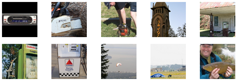
These are 10 images from the following Imagenet-1k classes: “cassette_player”, “chain_saw” (x2), “church”, “gas_pump” (x3), “parachute” (x2), and “tench”.

Real images.

Now that the images are loaded, let’s apply some lightweight pre-processing on them to use them for FID calculation.

Copied

from torchvision.transforms import functional as F


def preprocess_image(image):
    image = torch.tensor(image).unsqueeze(0)
    image = image.permute(0, 3, 1, 2) / 255.0
    return F.center_crop(image, (256, 256))


real_images = torch.cat([preprocess_image(image) for image in real_images])
print(real_images.shape)
# torch.Size([10, 3, 256, 256])

We now load the DiTPipeline to generate images conditioned on the above-mentioned classes.

Copied

from diffusers import DiTPipeline, DPMSolverMultistepScheduler

dit_pipeline = DiTPipeline.from_pretrained("facebook/DiT-XL-2-256", torch_dtype=torch.float16)
dit_pipeline.scheduler = DPMSolverMultistepScheduler.from_config(dit_pipeline.scheduler.config)
dit_pipeline = dit_pipeline.to("cuda")

words = [
    "cassette player",
    "chainsaw",
    "chainsaw",
    "church",
    "gas pump",
    "gas pump",
    "gas pump",
    "parachute",
    "parachute",
    "tench",
]

class_ids = dit_pipeline.get_label_ids(words)
output = dit_pipeline(class_labels=class_ids, generator=generator, output_type="numpy")

fake_images = output.images
fake_images = torch.tensor(fake_images)
fake_images = fake_images.permute(0, 3, 1, 2)
print(fake_images.shape)
# torch.Size([10, 3, 256, 256])

Now, we can compute the FID using torchmetrics.

Copied

from torchmetrics.image.fid import FrechetInceptionDistance

fid = FrechetInceptionDistance(normalize=True)
fid.update(real_images, real=True)
fid.update(fake_images, real=False)

print(f"FID: {float(fid.compute())}")
# FID: 177.7147216796875

The lower the FID, the better it is. Several things can influence FID here:

• Number of images (both real and fake)

• Randomness induced in the diffusion process

• Number of inference steps in the diffusion process

• The scheduler being used in the diffusion process

For the last two points, it is, therefore, a good practice to run the evaluation across different seeds and inference steps, and then report an average result.

FID results tend to be fragile as they depend on a lot of factors:

• The specific Inception model used during computation.

• The implementation accuracy of the computation.

• The image format (not the same if we start from PNGs vs JPGs).

Keeping that in mind, FID is often most useful when comparing similar runs, but it is hard to reproduce paper results unless the authors carefully disclose the FID measurement code.

These points apply to other related metrics too, such as KID and IS.

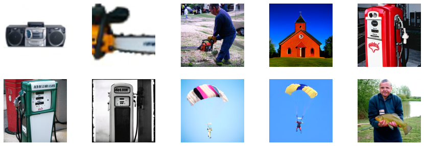
As a final step, let’s visually inspect the fake_images.

Fake images.